Help centre
How can we help you?
Guides and examples
In this section, you’ll find some guides and examples of how to construct SQL queries to produce some frequently needed reports, and how to access your data from common reporting tools to produce graphs and dashboards.
Namely, you’ll learn:
- How to build a query for a Volumes report
- How to use your data from Google Data Studio
- How to use your data from Tableau
Note that BigQuery provides two different flavors of SQL: legacy SQL and standard SQL. All the examples in this section are written using standard SQL. That’s the syntax we recommend our users use as well, as it is compliant with the SQL 2011 standard, and it provides extensions very helpful when making complex queries.
All the query examples in this section are using the wadus account. You’ll need to replace wadus with the name of your dataset for the queries to work.
Volumes report
A typical use case of Reporter is generating volumes reports. Usually, a volumes report shows how much content is scheduled platform by platform, month by month (or day, week, year…)
For instance, the following query will return the number of schedule entries going online (i.e., starting) each month on each platform in an account:
#standardSQL
select
  platform_name,
  format_timestamp("%Y-%m", schedule_entry_starts_at) month_key,
  count(*) going_online_entries

from
  wadus.schedule_entries
    inner join wadus.platforms using (platform_id)

group by 1, 2

order by 1, 2
Interesting remarks about this query:
- The data we need lives in the
schedule_entriestable. We need to join that one with theplatformstable to get each platform’s name. - We’re using the
usingclause when joining tables. That clause is equivalent toon schedule_entries.platform_id = platforms.platform_id, but much shorter.
Now, let’s say that, instead of counting the number schedule entries, we want to know the total number of hours of content that start each month:
#standardSQL
select
  platform_name,
  format_timestamp("%Y-%m", schedule_entry_starts_at) month_key,
  round(sum(version_runtime_in_ms) / (1000 * 60 * 60)) going_online_hours

from
  wadus.schedule_entries
    inner join wadus.platforms using (platform_id)
    inner join wadus.versions  using (version_id)

group by 1, 2

order by 1, 2
We did two things here:
- We added a new
joinclause to thefromexpression, theversionstable; this gives us the title version used by each schedule entry, and that’s where we will find the runtime of the title. - We summed the
version_runtime_in_ms(from theversionstable) in theselectexpression. Since that field returns the runtime of the version in milliseconds, we divided that value by(1000 * 60 * 60)to convert it to hours.
Now, the two queries before have one limitation: if a given platform in a given month doesn’t have any schedule entry, then that platform/month combination won’t appear in the results; and this might not be what we want. Usually, in that scenario, we want the platform/month combination to appear in the results but with a 0 as the number of going online entries. The following query gets us what we want:
#standardSQL
with
  months as (
    select format_date('%Y-%m', month_start) month_key
    from unnest(
      generate_date_array('2016-01-01', '2016-12-01', interval 1 month)
    ) month_start
  )

select
  platform_name,
  month_key,
  count(schedule_entry_id) going_online_entries

from
  wadus.platforms
    cross join months
    left join wadus.schedule_entries
      on platforms.platform_id = schedule_entries.platform_id
     and format_timestamp("%Y-%m", schedule_entry_starts_at) = month_key

group by 1, 2

order by 1, 2
Ok! Things are getting interesting:
- First of all, we’re generating a temporary table called
monthsusing thewithclause. This clause allows us to generate a table with the contents of the given subquery and that will only exist during the execution of the query. - The temporary
monthstable contains one row per month within 2016. To generate such a table, check out how theunnestclause and thegenerate_date_arrayfunction work. - In the
fromclause, first of all, we’re doing a cross join between all the platforms and all the months. That’s to ensure every platform/month combination will be listed. - The platforms/months cross join is then joined with our
schedule_entriestable, by both the platform and the start date of each entry.
Finally, let’s say that, instead of the content going online (i.e., starting) every month, we want to count the number of entries online every month (i.e., entries that start that month or before and end that month or after).
With a minor change over our previous query we can get exactly that:
#standardSQL
with
  months as (
    select format_date('%Y-%m', month_start) month_key
    from unnest(
      generate_date_array('2016-01-01', '2016-12-01', interval 1 month)
    ) month_start
  )

select
  platform_name,
  month_key,
  count(schedule_entry_id) online_entries

from
  wadus.platforms
    cross join months
    left join wadus.schedule_entries
      on platforms.platform_id = schedule_entries.platform_id
     and format_timestamp("%Y-%m", schedule_entry_starts_at) <= month_key
     and format_timestamp("%Y-%m", schedule_entry_ends_at)   >= month_key

group by 1, 2

order by 1, 2
We just needed to change the conditions on how the months table joins with the schedule_entries table to reflect this.
And now that we have our query ready, we may want to use it in our reporting solution. In the following sections, you’ll learn how to create a report in Google Data Studio and Tableau based on the last query above.
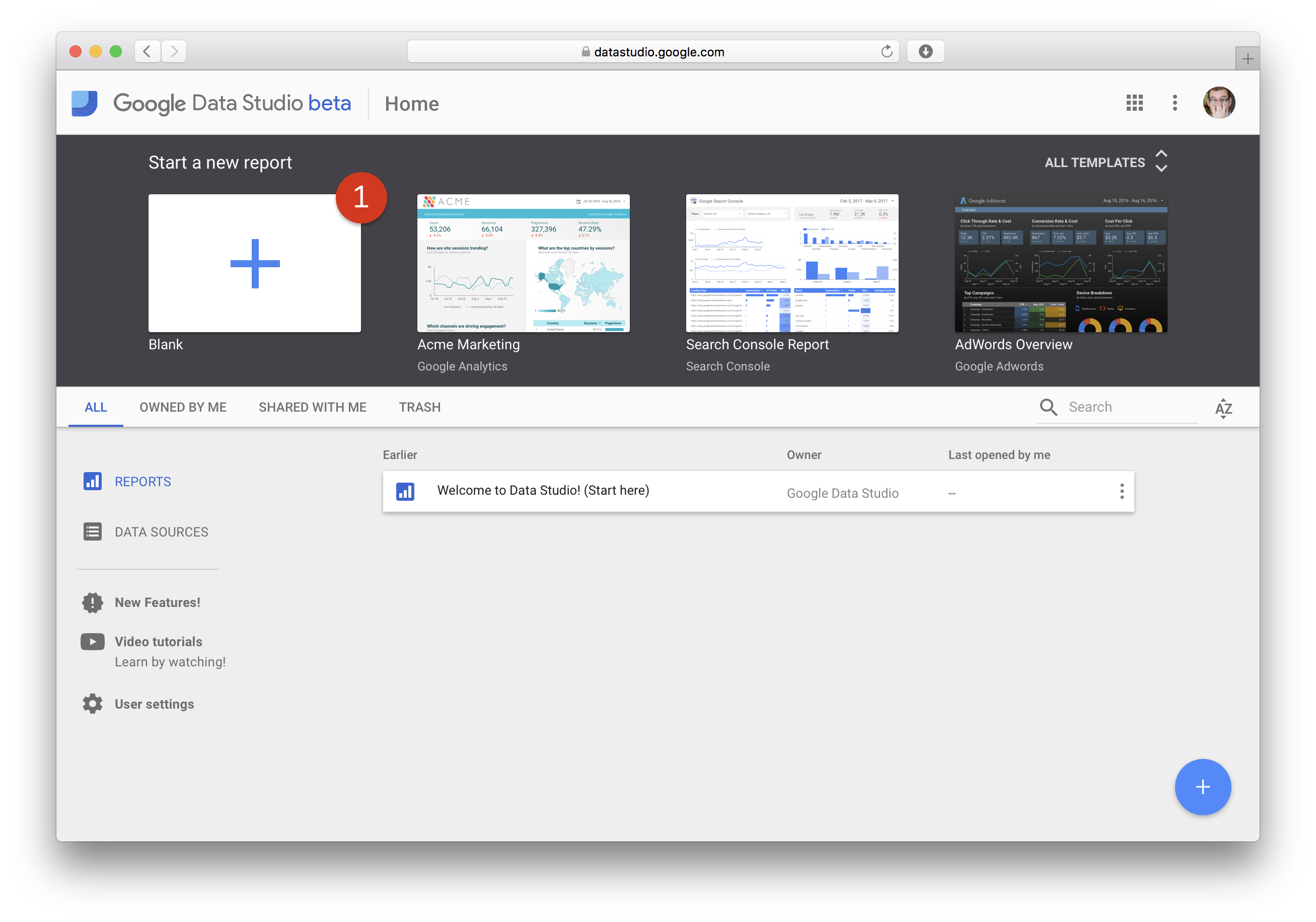
Reporting from Google Data Studio
To use Google Data Studio, you’ll need a Google User Account with access to your dataset. Please ask Mediagenix On-Demand Support or your TAM if you need one.
Once you visit datastudio.google.com and enter your Google credentials you’ll see the tool’s welcome screen. We can start creating our first report by clicking on (1):
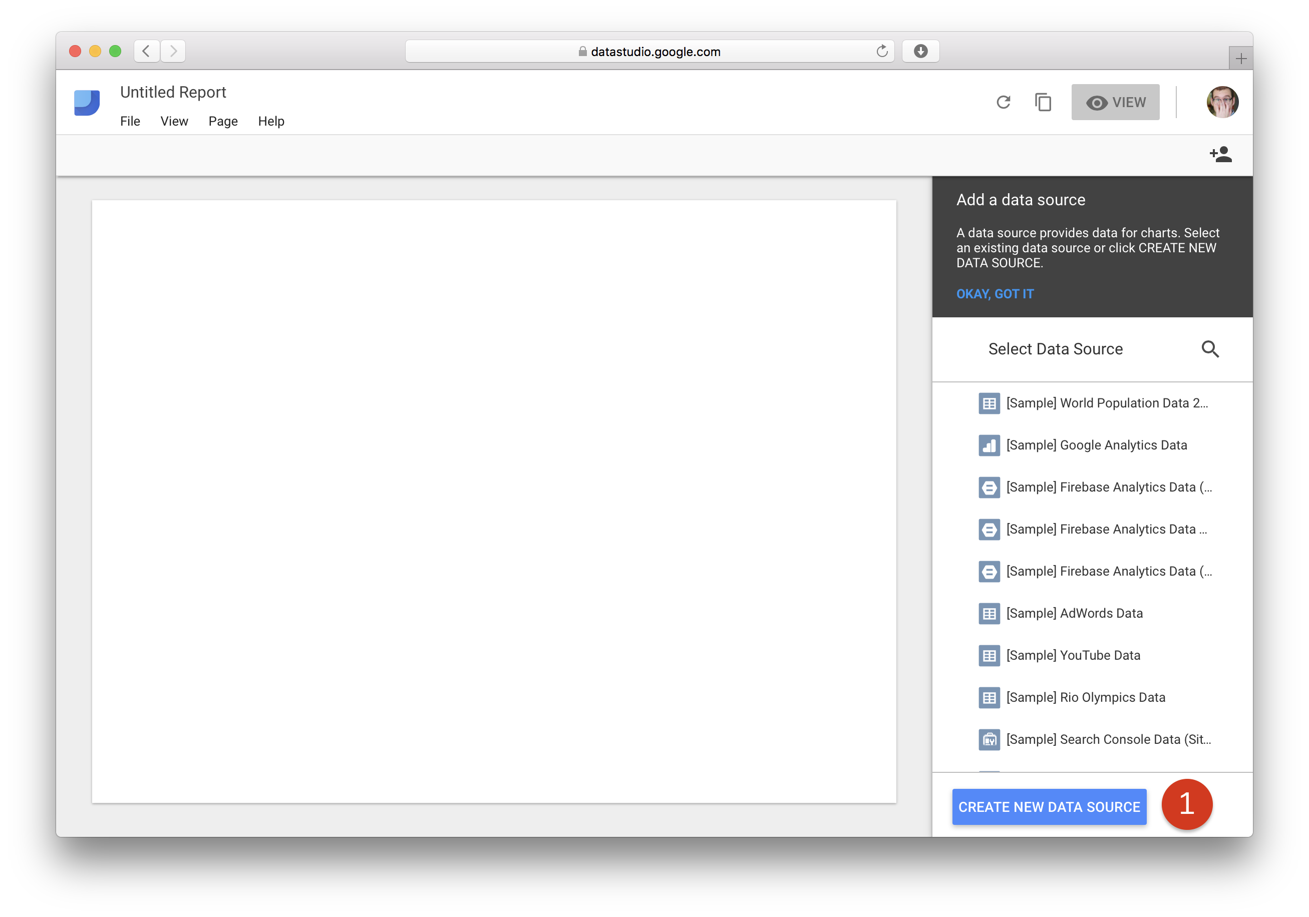
We first need a data source, so we’ll create a new one (1):
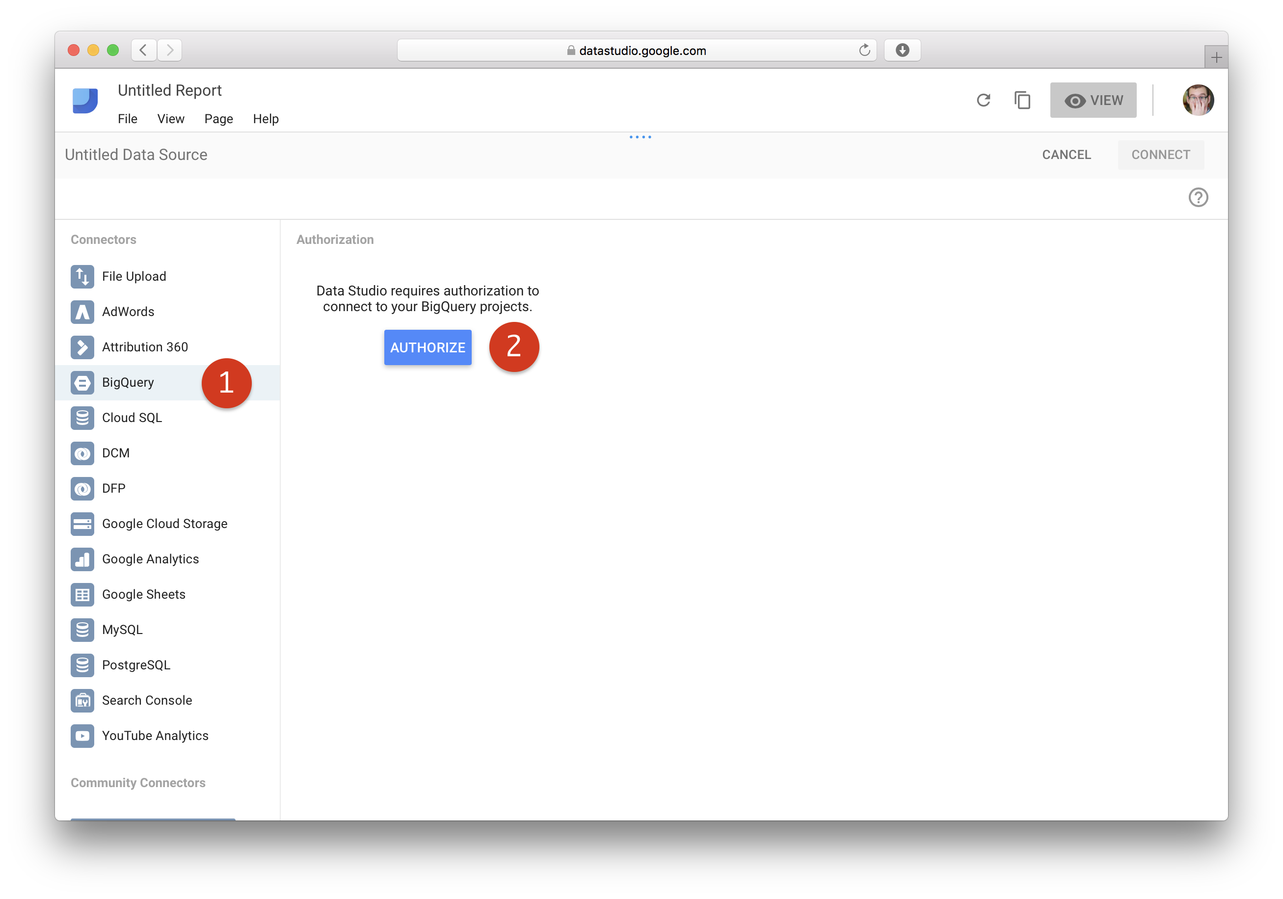
In the “Connectors” section we need to pick “BigQuery” (1). Then, if this is our first time using Data Studio, we need to authorize access to BigQuery (2):
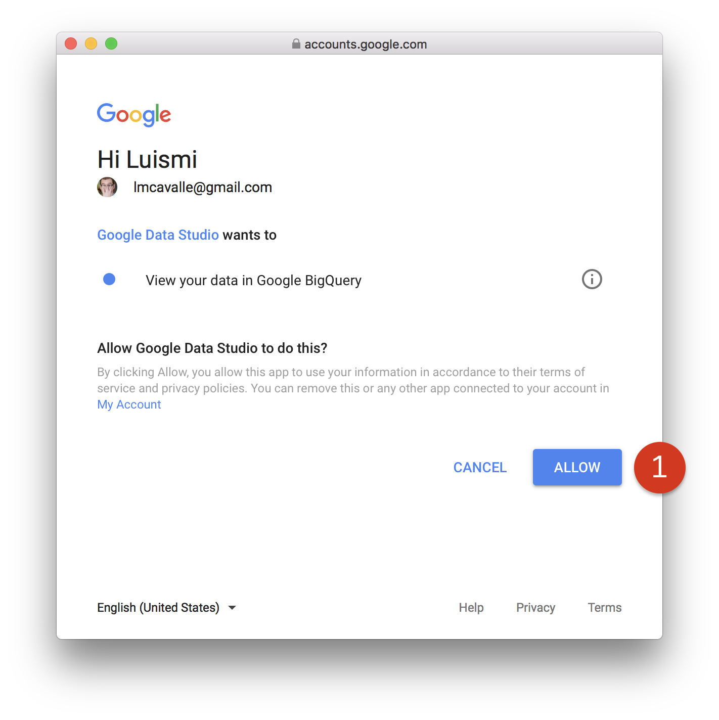
A pop-up will appear showing a series of screens to allow Data Studio to access our BigQuery account (1):
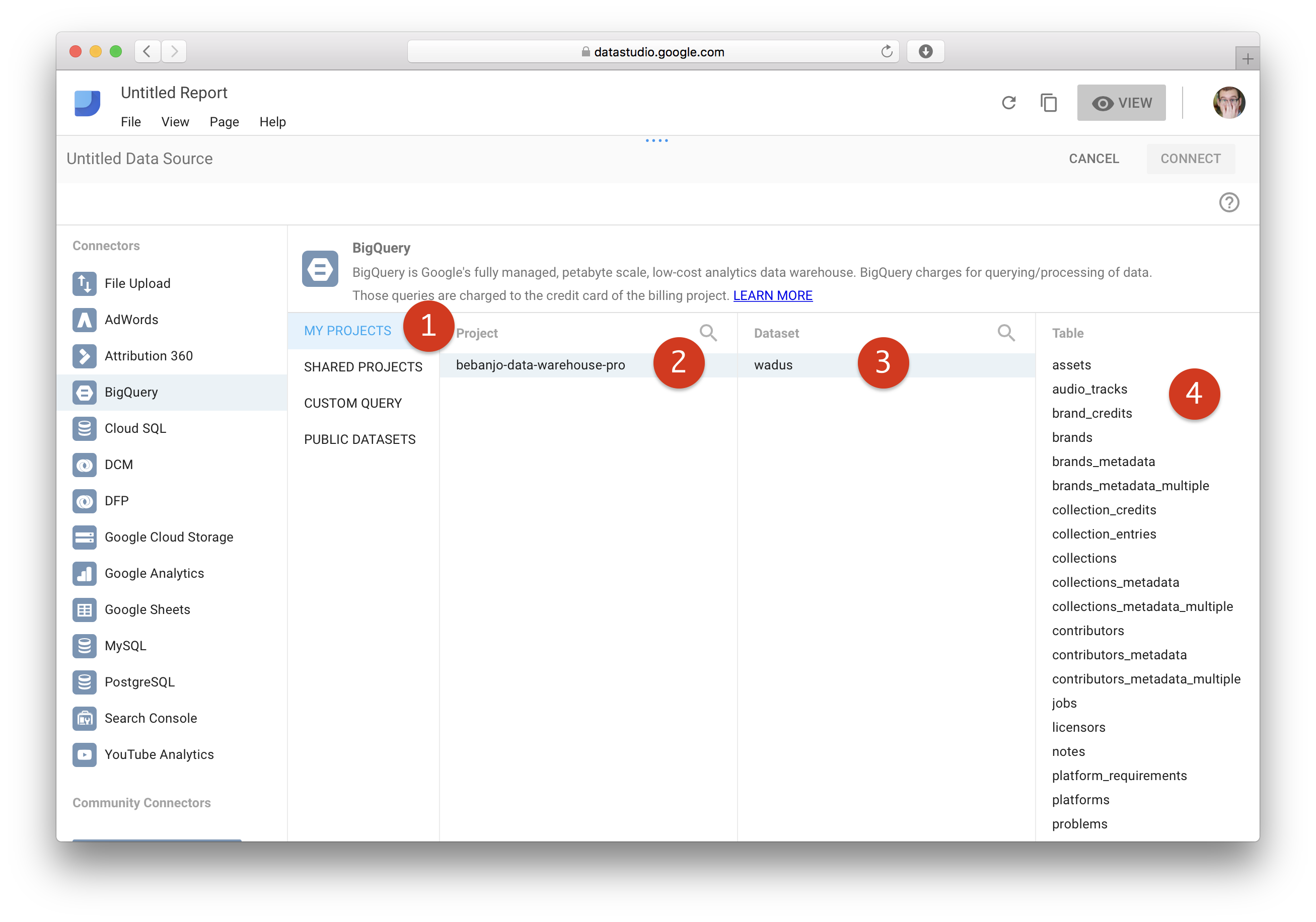
Now, clicking on “My projects” (1) we should see our project (2) and then our dataset (3); this would allow us to pick any of the tables in our Reporter dataset (4):
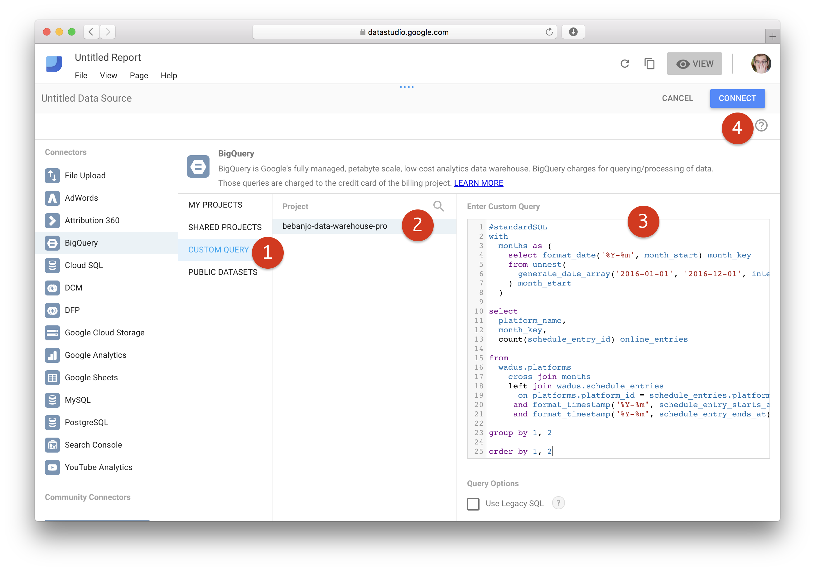
However, in this case, we want to use a custom query. So, we click “Custom query” (1) and then our project (2). Now we can enter any query we want. In this case, we’re going to use one we saw in the previous section (3). To continue, we click “Connect” (4):
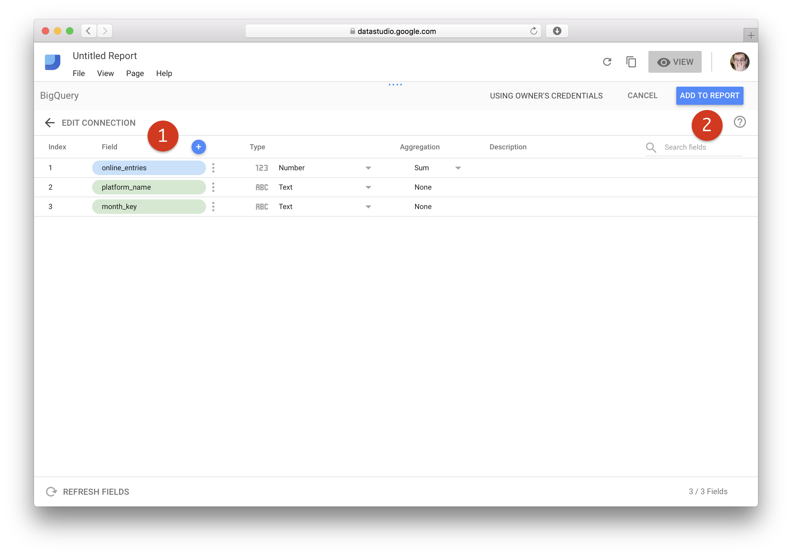
At this screen, we can review that the fields of our query became available (1), and continue by clicking on “Add to report” (2):
We might be requested to allow additional access to Data Studio the first time we use it. We just need to allow it (1):
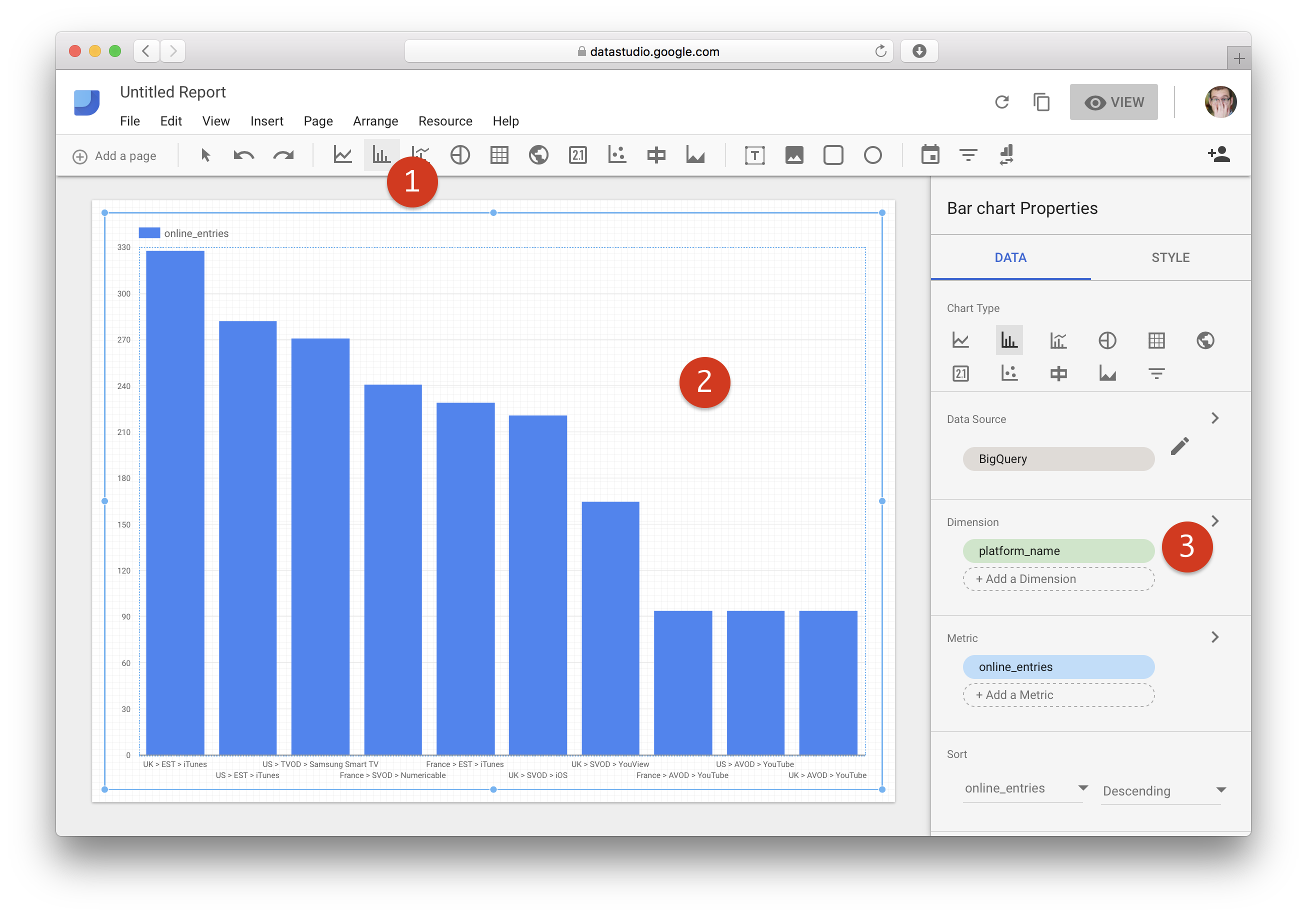
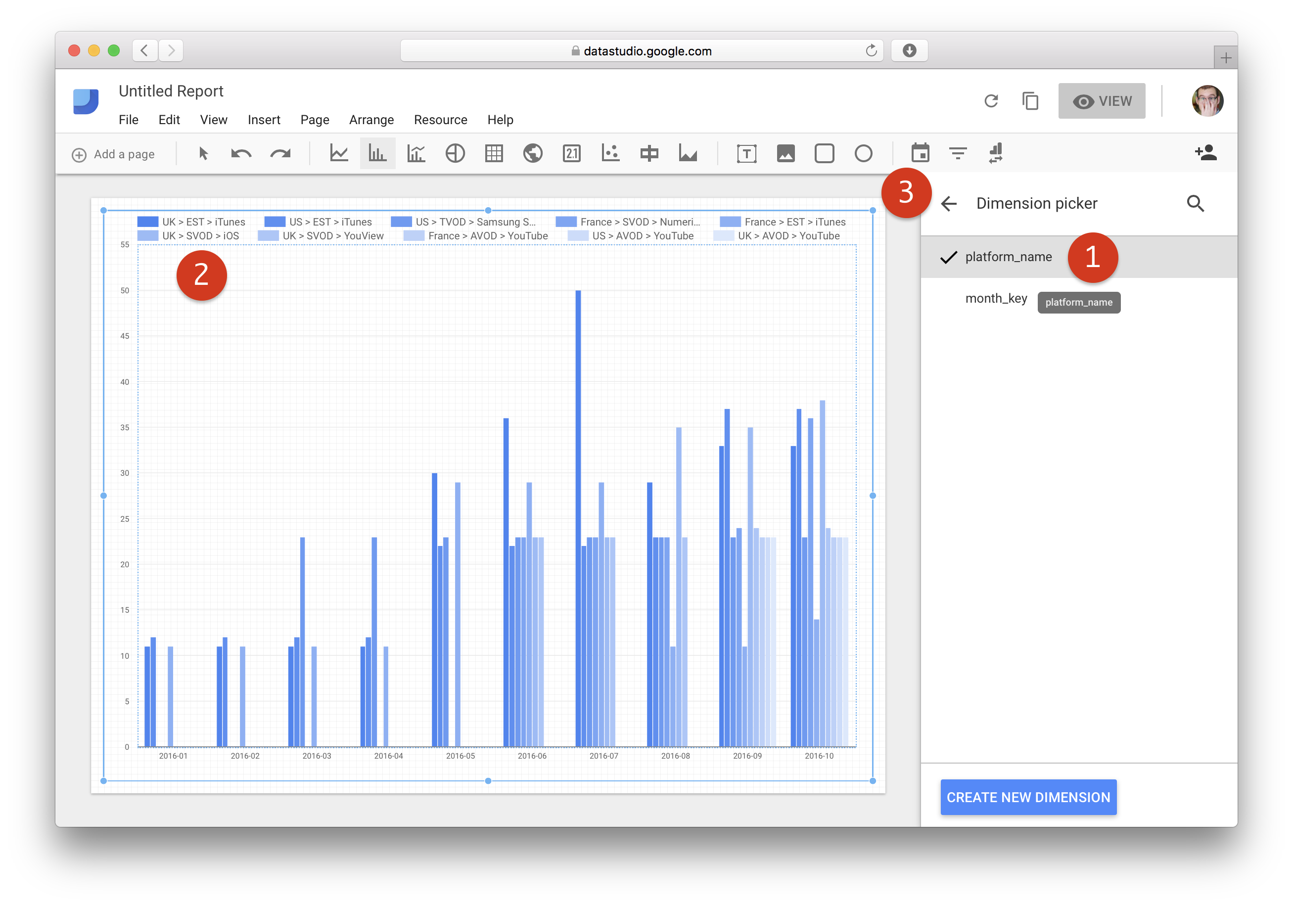
Now, we can create our report. We click on the “Bar chart” icon (1), and then drag and drop a rectangular area in the canvas (2). This graph shows one bar per platform, however, what we want is one bar per month, so we click on platform_name in the “Dimensions” section (3):
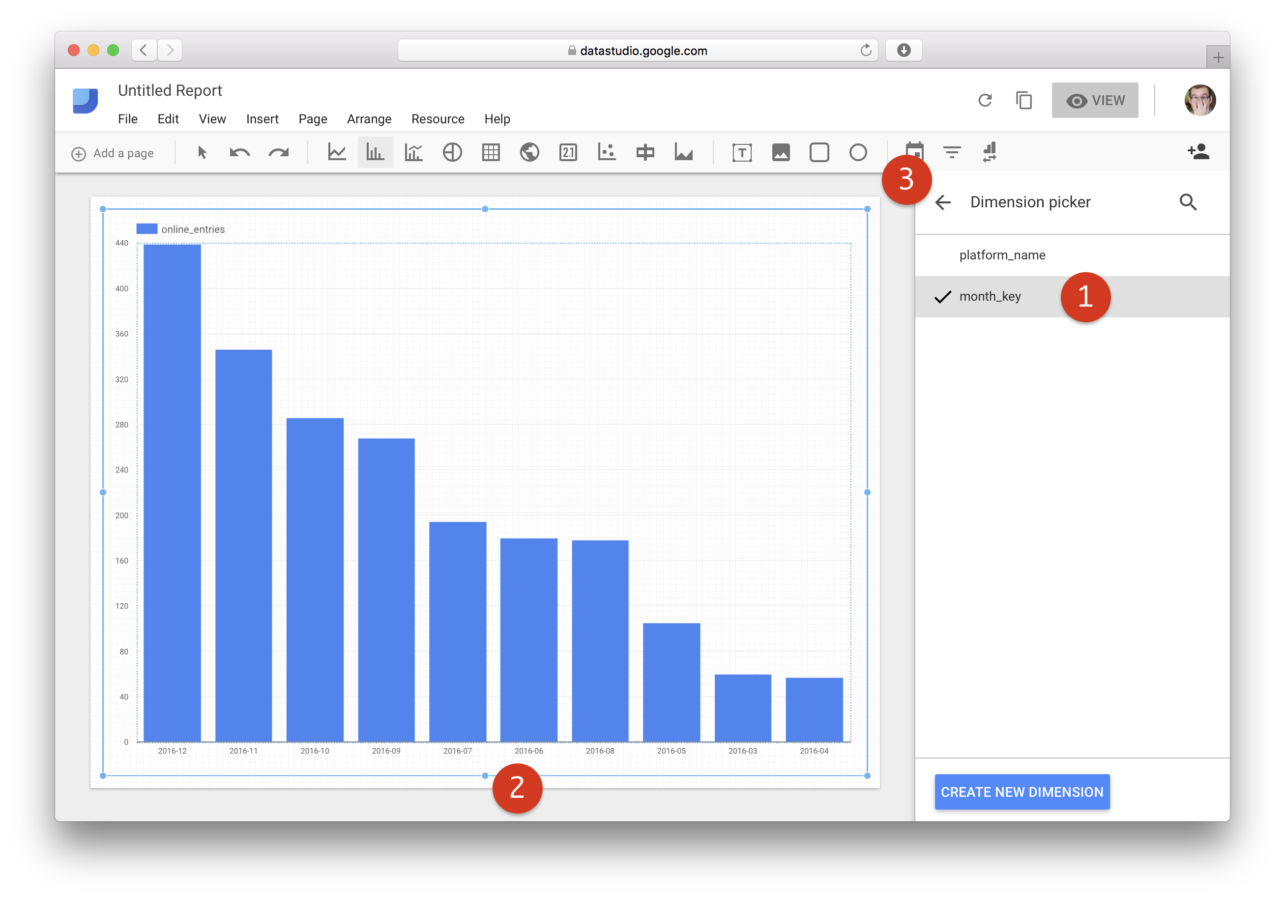
Now we choose the month_key (1); this will get us what we want (2). We can now go back (3):
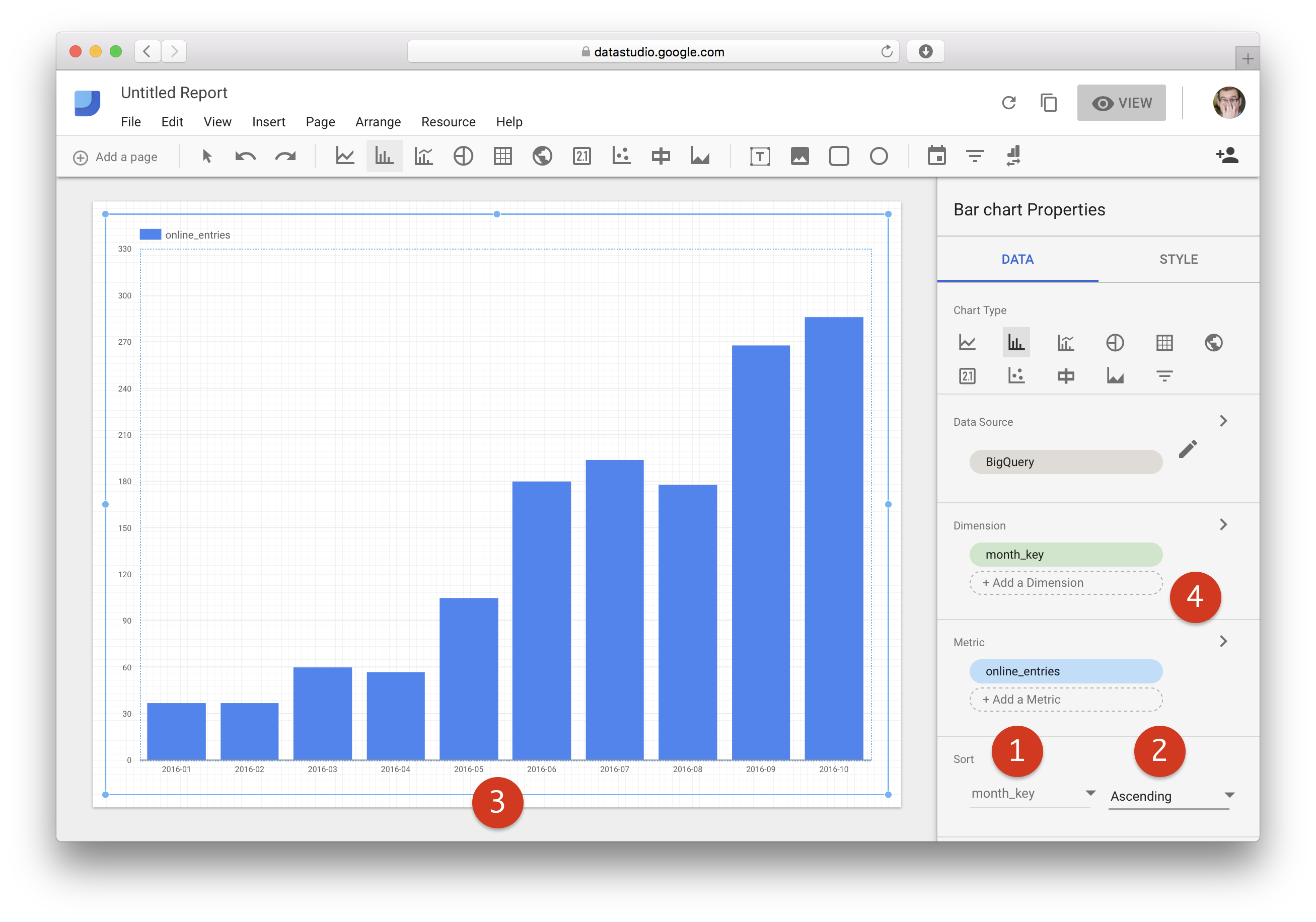
At this point, we need to set the proper order in the bars. We change the sorting to month_key (1) ascending (2). That will sort the bars properly (3). Next, we’ll add another dimension (4):
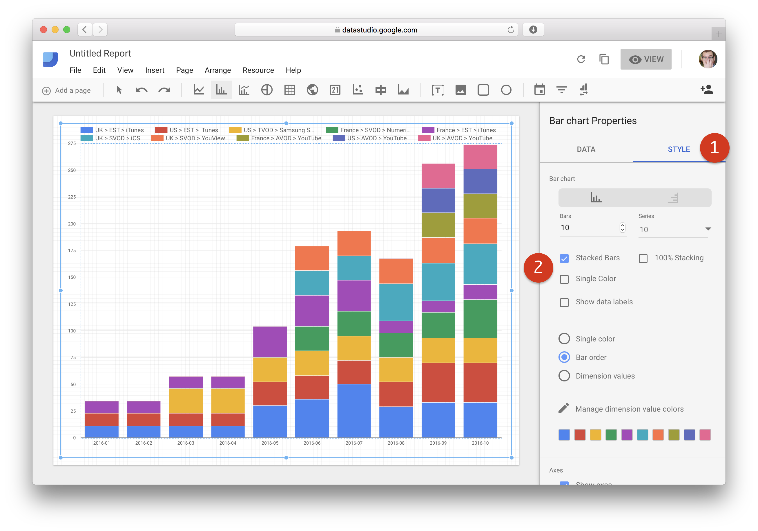
We’ll pick the platform_name now (1); this will show one bar per platform and month (2). We can go back now (3):
Finally, we go to the “Style” tab (1), check “Stacked Bar” and uncheck “Single Color” (2), and our report is ready!
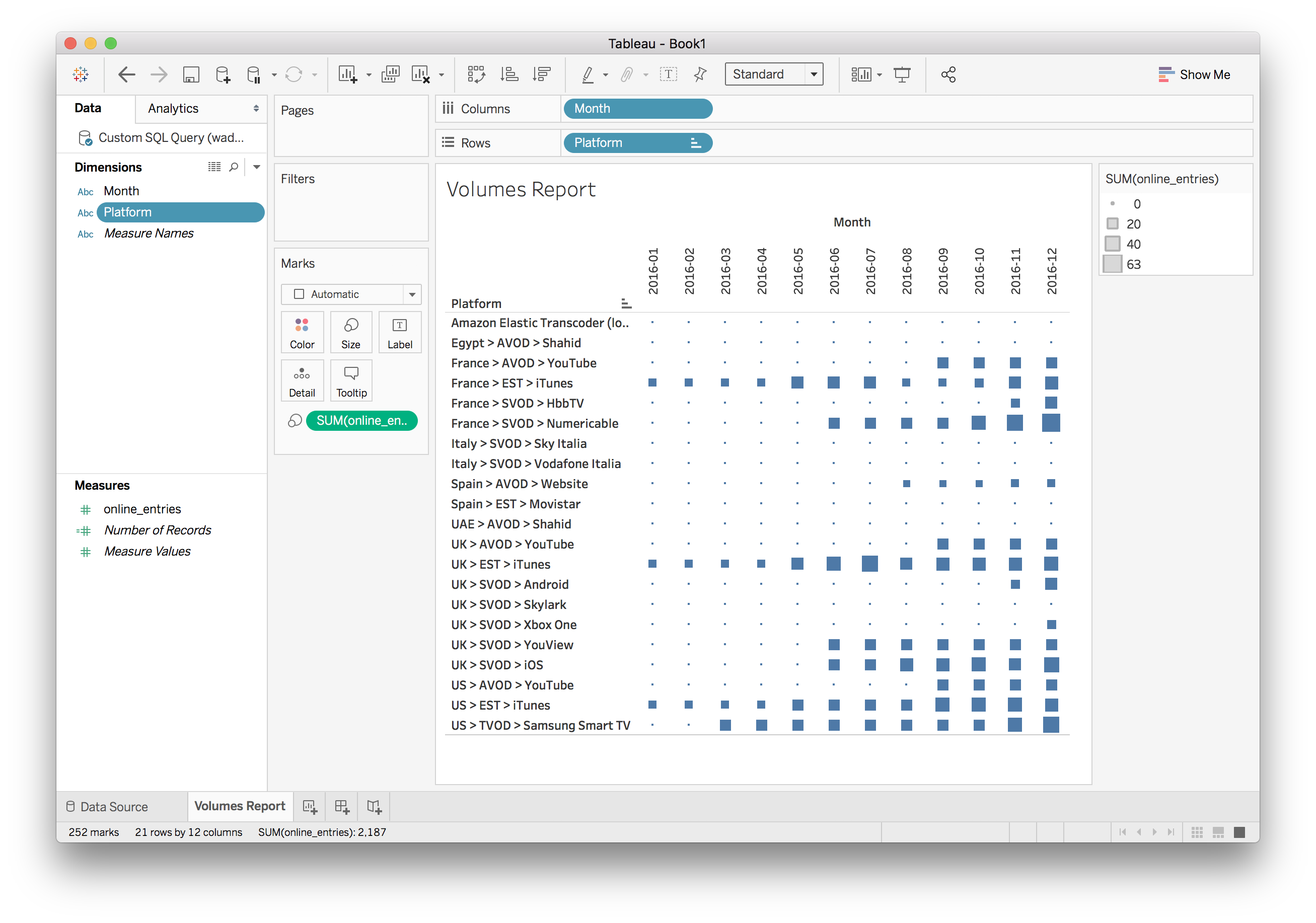
Reporting from Tableau
To use Tableau, you’ll need a Google User Account with access to your dataset. Please ask Mediagenix On-Demand Support or your TAM if you need one.
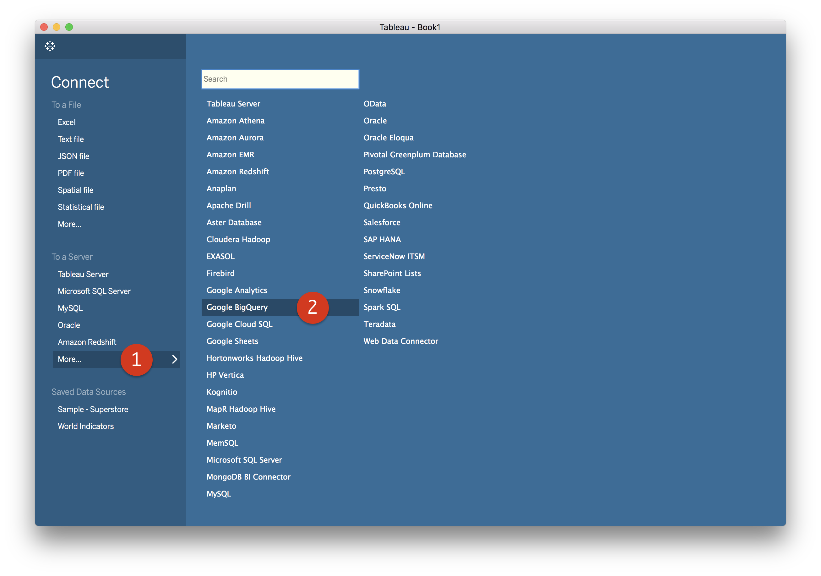
First, from the “Connect” screen of table we need to click on “More…” within “To a Server” (1) and then choose “Google BigQuery” (2):
A pop-up will show up with a series of screens. We will need to enter our Google credentials here to allow the tool to access our data in BigQuery (2):

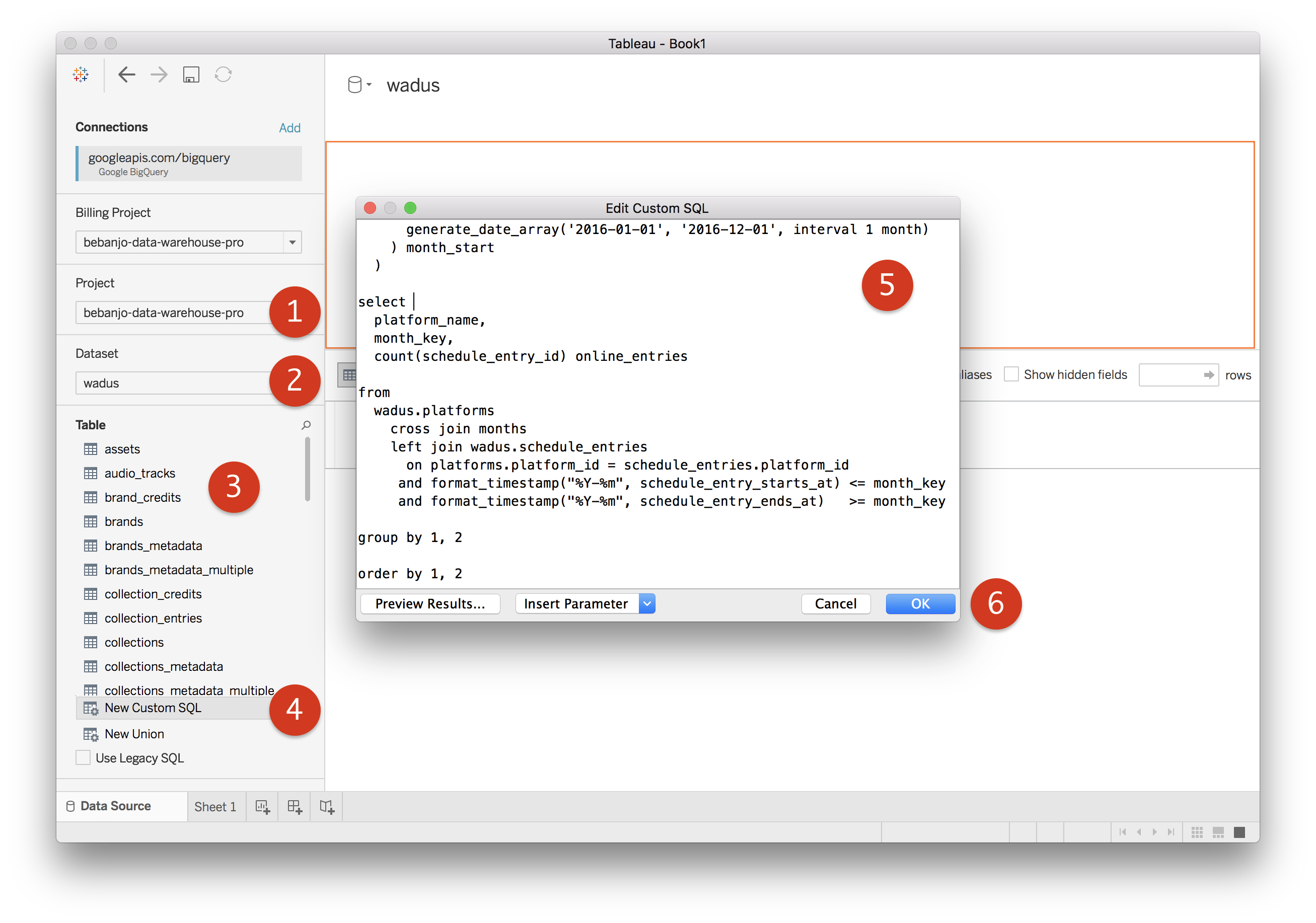
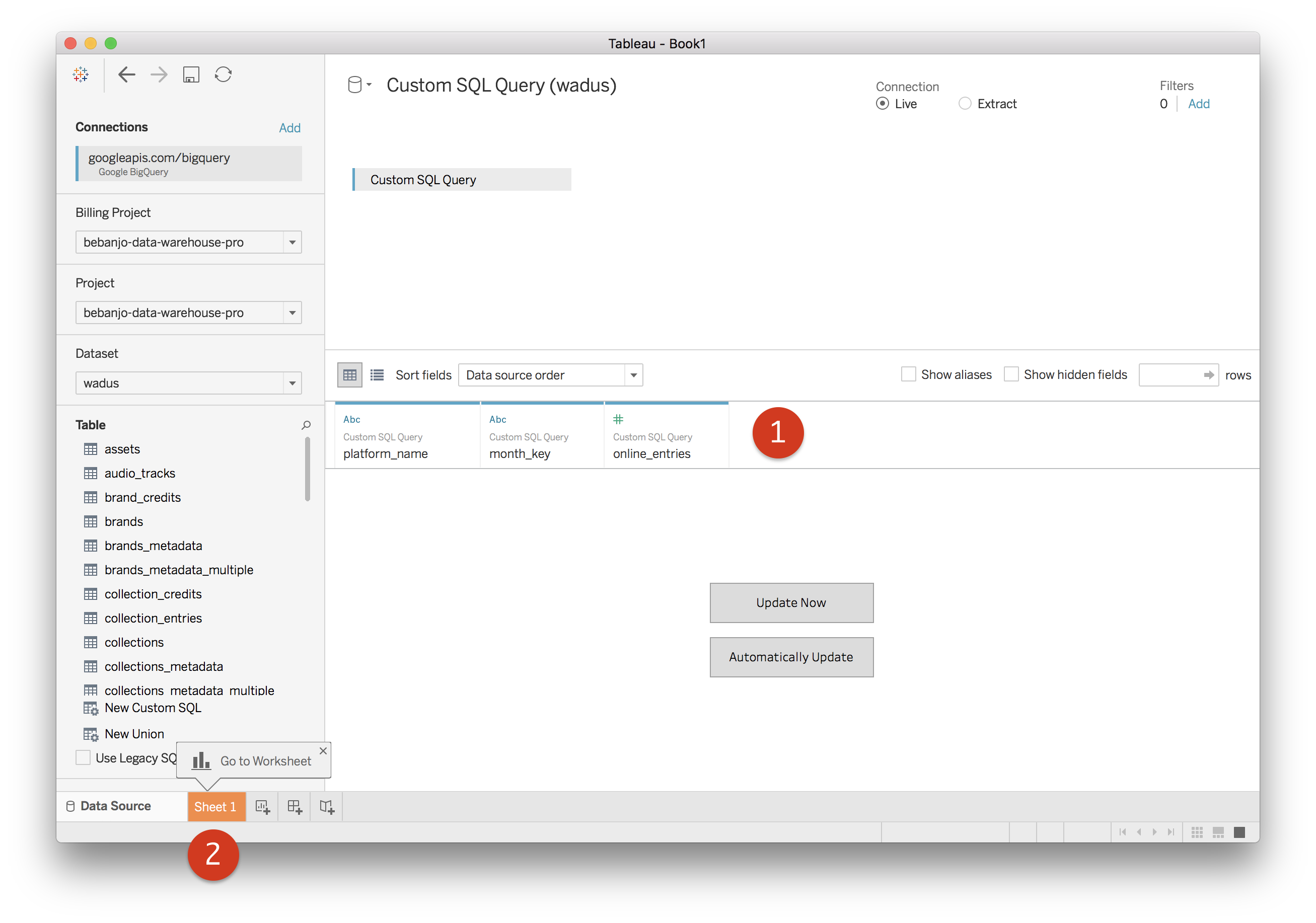
Now, we need to select our BigQuery project (1) and our dataset (2). We can then drag and drop any of the tables in the dataset to use them as our source of data (3). However, instead of that, we’ll drag and drop “New Custom SQL” (4) which will allow us to enter a custom query (5). In this case, we’re going to use one we saw in the previous section. To continue, we click “OK” (6):
At this point, we can review that the fields of our query became available (1), and then continue to our first sheet (2):
Within the sheet editor, we’ll first select, keeping the shift key pressed, the two dimensions (1) and the measure (2) of our data source; this will enable us to select the “Heat map” report (3). Then, we will switch the month_key and the platform_name (4) as we want the platforms to appear as rows and the months as columns:
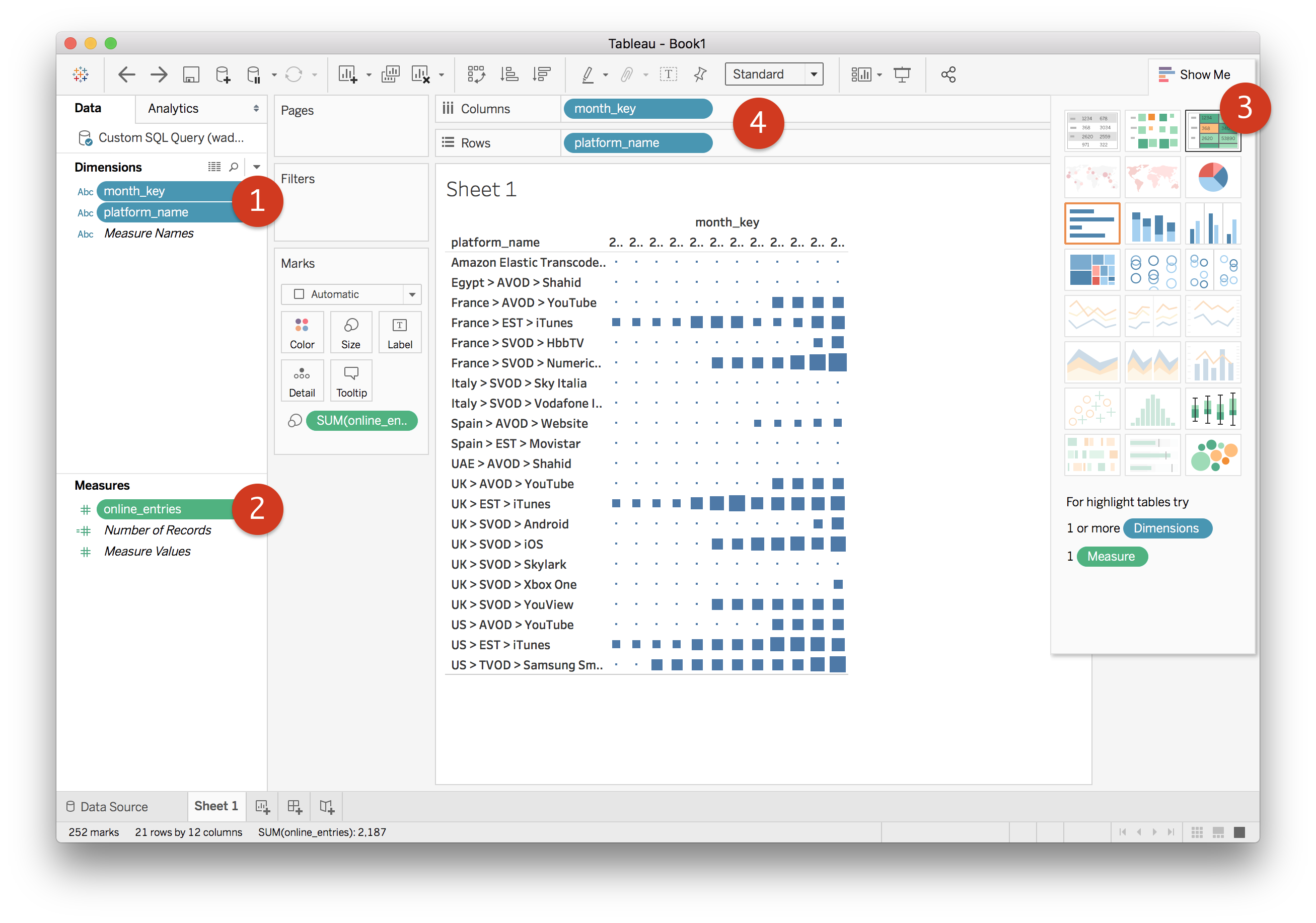
Now, we only need to fix a bit the formatting and the labels, and our Tableau report is ready!